Estimated Required Reading Time: 10 minutes
In distribution operations defect rates on products that have been shipped to customers are measured as a ratio of defects divided by total products shipped, to normalize for shipping volume.
One common method for measuring defect rates is to divide the defects reported in a period by the number of shipments from the same period. Although commonly used, the method is invalid because the defects haven’t occurred in the same period as the shipment. Not only is the data by period incorrect, the method will also fail to show a valid trend over time. The reason? Defects in products shipped last month, are not correlated with the volume of products shipped this month, so volume hasn’t been normalized, which is the purpose of using a ratio instead of the actual number of defects.
For example, ten defects in a month with 1,000 shipments isn’t the same failure rate as ten defects in a month with 100 shipments. Normalizing the data for volume is the remedy – dividing defects by shipments. But if the defects are reported in the current period that were a result of shipments in a prior period, then using a ratio to normalize for volume doesn’t give valid data – the shipment period and the defect period must match. To extend the above example, if the ten defects from a period with 1,000 shipments are reported against the 100 shipments in the subsequent period, the defect rate will be erroneously reported as 10% — instead of the correct rate of 1%.
To recognize a valid trend, without going back in time and matching defects to their respective data periods, the ratio can be calculated using cumulative data. For example, each month’s shipments and defects can be added to the previous month’s shipments and defects to calculate a running average rate of defects. The weakness of that model is that a change in data trends will take considerable time to emerge because of the weight of the previous period’s data in the calculation. Limiting the effect of weighting can be mitigated by limiting the time fence: for example, using a one-year running average. Still, there will be a significant lag, and suppression of the magnitude of change when it occurs.
A second method for determining defect rates is to use a statistical model, in which a hundred orders (as an example) are chosen at random from a past period and matched with defect reports specific to individual orders in the sample set. The weakness of that method is that it does not consider defects from the sample period that have yet to be reported.
The most valid method of tracking rates of defects is to maintain an evergreen reporting system where defects are assigned to their period of production, which results in continuously updating the quality metrics bringing trends into sharper focus over time.
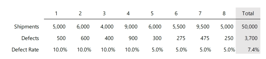
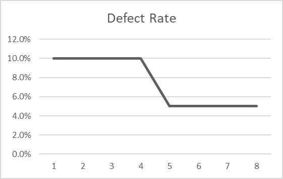
Example: For four consecutive periods, a company ships between 5,000 and 10,000 orders per period and consistently experiences a 10% defect rate. After four periods, the company makes an improvement that reduces defects by half, resulting in a 7.4% weighted average defect rate over the eight periods. When the defects are matched to the shipment period, the frequency distribution looks like:
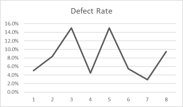
If the defect numbers are shifted one period into the future, which is to say, the defects from orders shipped are reported the next month, the data and trend from the exact same data set become nonsensical.

An additional challenge is determining root cause using defect rates. For example, comparing defects to the date of the shipment doesn’t account for the actual date of manufacturing if the product was in inventory, causing the same data fallacy discussed above. If the root cause of the defect is a component manufactured by others, the same data fallacy occurs unless each defect can be matched to the date the supplier made the error.
What to look for in the data: When examining defect rates, it is helpful to measure the variance across the data. In normal frequency distributions, 68% of the data will be one standard deviation from the mean – or have a Z-score between -1 and 1. When data sets show wild swings in defects, in processes that have been standardized, there is a good chance the metric isn’t valid, or a random element has been introduced into the process. When the defect, and production dates are matched, the data over time will present as a normal curve (bell shaped) with 34% of the data on either side of the mean.
Take-away: Defect rates are tricky to calculate, especially for large data sets, with layers of possible root cause, and lag time between production of the defect, and reporting of the defect. Often the root cause of defects is best addressed empirically – such as performing forensic and root-cause analysis on defective samples. Looking at 12-month weighted average rates of defects requires taking the long view but has the advantage of self-correcting for mismatched reporting periods.